Tracking
Open the workflow in NIS-Express:
Tracking connects the “same” objects or particles across time-lapse sequences. Because objects may appear, disappear, divide, or change shape between frames, they typically receive different object IDs on each frame. Tracking solves this by assigning each object a persistent track ID that remains constant across frames for the same physical entity.
Overview of tracking methods
GA3 provides two distinct tracking approaches optimized for different applications:
Object tracking
Track Objects is designed for larger, morphologically complex objects like cells. It:
- Works directly with binary layers
- Uses object frame-to-frame overlap to assign track ID
- Handles objects that change shape between frames
- Combines easily with standard object measurements
- Is suitable when objects are morphing over time
Use for: Cells, organoids, cell clusters, tissue regions
Particle tracking
Track Particles is optimized for point-like particles and includes motion modeling:
- Works with centroid positions (not binary layers)
- Uses position-based algorithms with motion prediction
- Offers different motion models (Brownian, directed)
- Provides specialized motion analysis features
- Handles high particle densities efficiently
- Is suitable for small/rigid bodies
Use for: Vesicles, fluorescent spots, small organelles, diffusing molecules, single particles
This guide covers three complete tracking workflows demonstrating both approaches:
- Track moving objects - Object tracking combined with morphology measurements
- Particle tracking with motion analysis - Motion feature calculation and motility classification
- Single particle tracking with diffusion - Mean squared displacement (MSD) and diffusion coefficient analysis
Common workflow structure
All tracking workflows share a similar pipeline structure:
Segmentation
Detect objects or particles in each frame independently using appropriate segmentation methods.
Position measurement
Extract time and position information for each detected object.
Required for particle tracking
Tracking algorithm
Connect objects/particles across frames using either Track Objects or Track Particles node.
Append Object measurement (optional)
Append object/cell measurements to the track IDs.
Typical for object tracking
Track accumulation
Collect all tracking data across the entire time-lapse using Accumulate Tracks, filtering for minimum track length.
Analysis and visualization
Calculate motion features, display trajectories, and present results in synchronized views.
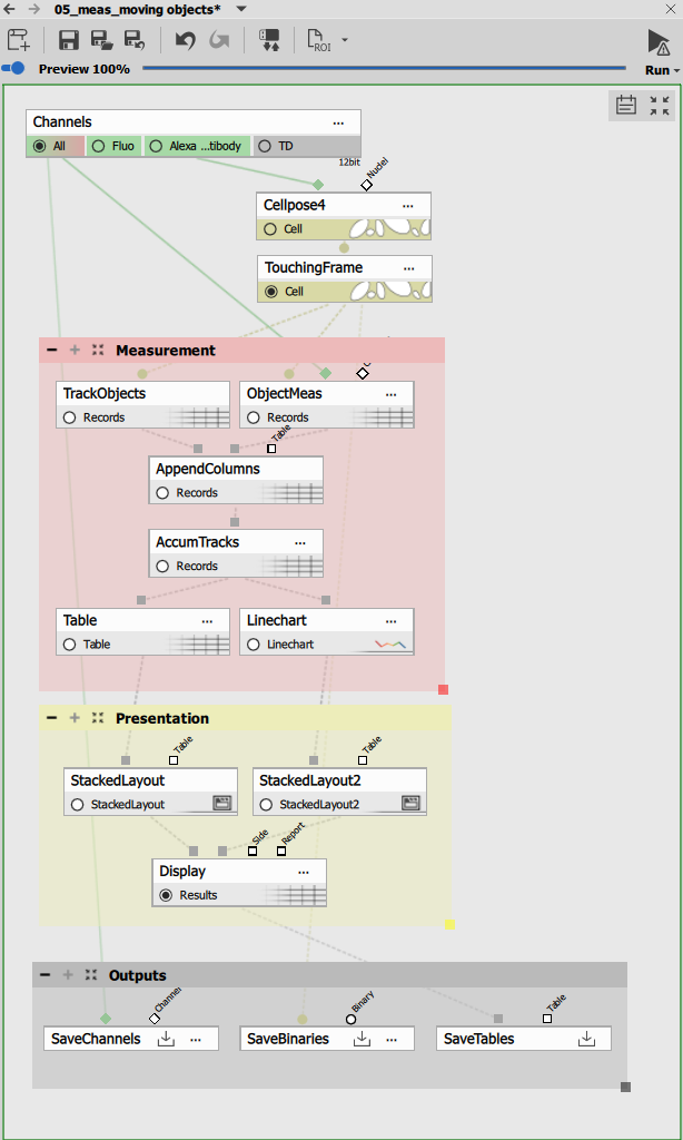
Workflow 1: Track moving objects
This workflow tracks cells or large objects while simultaneously measuring their morphological features.
---
config:
  look: handDrawn
  theme: neutral
---

graph TD
  subgraph "Tracking & Measurement"
    track[Track Objects]
    measure[Object Features]
    append[Append Columns]
    accum[Accumulate Tracks]
    chart[Line Chart]
    table[Table]
  end

  subgraph "Presentation"
    layout1[Stacked Layout - Left]
    layout2[Stacked Layout - Right]
    display[Display]
  end

  subgraph Outputs
    savechn[Save Channels]
    savebin[Save Binaries]
    savetab[Save Tables]
  end

  %% Main workflow
  channels[Channels] -->|Alexa 488| cellpose[Cellpose AI] -->|Cell| remove[Remove Touching Frame] -->|Cell| track
  remove -->|Cell| measure
  channels -.->|All| measure

  track -->|Records| append
  measure -->|Records| append

  append -->|Records| accum
  accum -->|Records| chart
  accum -->|Records| table

  %% Presentation
  chart --> layout2
  table --> layout1
  layout1 --> display
  layout2 --> display

  %% Outputs
  channels -->|All| savechn
  remove -->|Cell| savebin
  display -->|Results| savetab
Segmentation with Cellpose
Cellpose provides AI-powered cell segmentation on the fluorescent channel. The diameter parameter (35 pixels) is tuned for the typical cell size in the sample.
Border object removal
Remove Objects Touching Frame eliminates objects that touch the image border (5 pixel margin on all sides). This prevents tracking partial objects that enter or leave the field of view.
Object tracking
Track Objects assigns track IDs by matching objects between consecutive frames based on:
- Overlap between object positions
- Similarity in size and shape
- Proximity when objects don’t directly overlap
The output is a Records table with:
- TrackId: Persistent identifier for each tracked object
- Frame information: Time points where the object appears
- Object ID: Per-frame object number (changes each frame)
Object measurement
Object Features measures morphological and intensity features for each tracked object:
- Size: Area, perimeter
- Shape: Circularity, elongation, width, height
- Intensity: Mean, min, max, standard deviation in all channels
- Position: Centroid X, Y coordinates
Combining tracking with measurements
Append Columns merges the track IDs from Track Objects with the measured features from Object Features. Both tables have the same rows (one per object per frame), making the combination straightforward.
This creates a unified table where each object has:
- Its morphology and intensity measurements
- Its track ID linking it across time
- All temporal information
Track accumulation and filtering
Accumulate Tracks collects tracks across all frames with filtering:
- MinSegmentCount: 3 frames minimum
- Tracks appearing in fewer frames are discarded as transient noise
The accumulated data organizes objects by track, enabling temporal analysis of individual cells throughout the time-lapse.
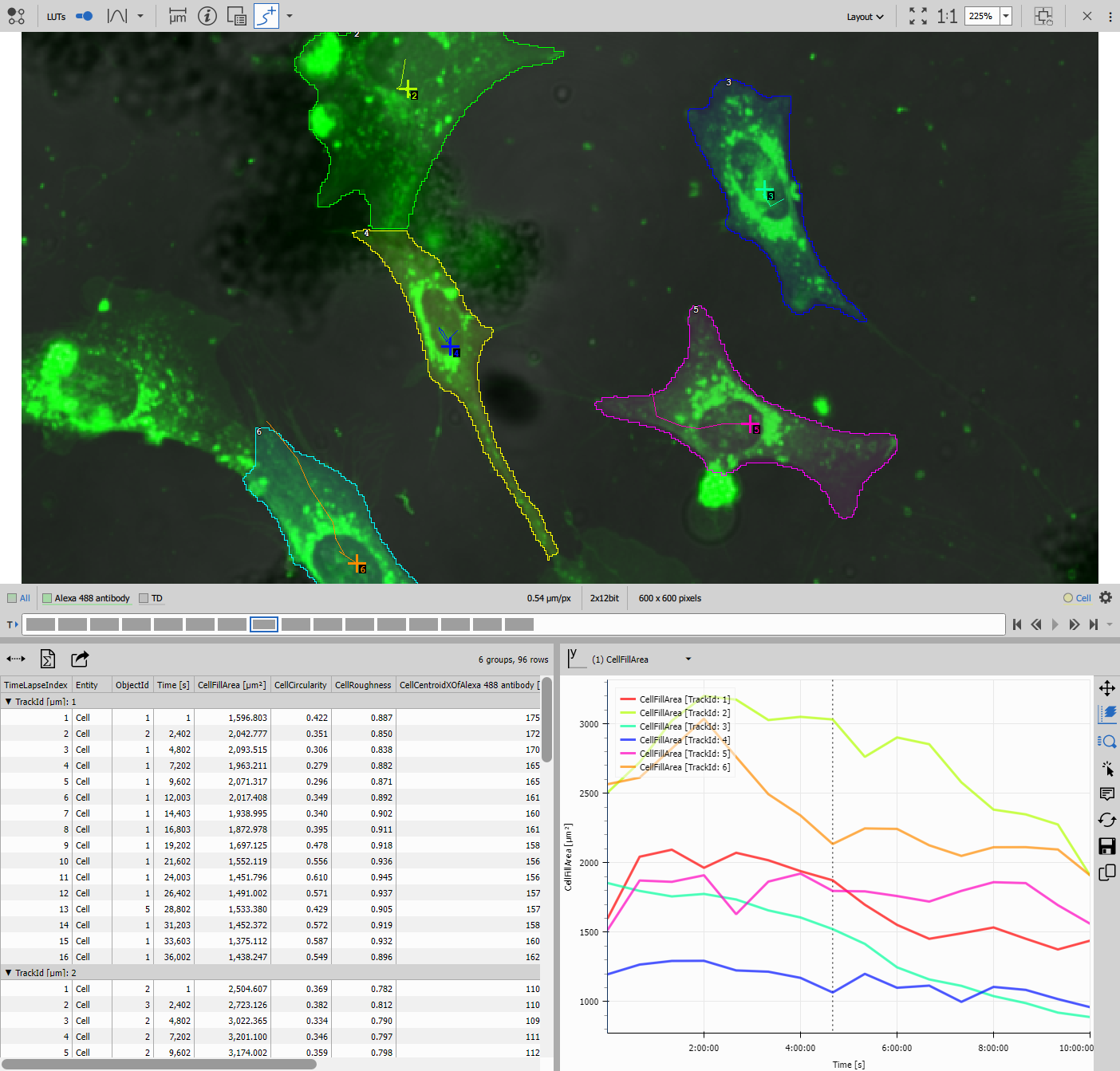
Visualization
Line Chart displays trajectories color-coded by track, showing how each cell moves over time. The chart can plot any measured feature vs. time (area changes, intensity variations, etc.).
Table shows all tracks with measurements at each time point, allowing sorting by track ID or any measured parameter.
Results
This workflow produces:
- Track IDs linking objects across time
- Complete morphological measurements for each tracked object
- Trajectory visualizations
- Combined segmentation masks and measurement tables
Use cases: Cell migration tracking, cell growth analysis, morphology changes during differentiation, long-term single-cell analysis
Workflow 2: Particle tracking with motion analysis
This workflow focuses on motion characterization, classifying particles by their motility patterns and measuring detailed motion features.
---
config:
  look: handDrawn
  theme: neutral
---
graph TD

  subgraph "Tracking Pipeline"
    time[Time and Center]
    track[Track Particles]
    accum[Accumulate Tracks]
    motion[Motion Features]
    rolling[Rolling Average]
  end

  subgraph "Motion Analysis"
    trackfeat[Track Features]
    calc[Create Column]
    group[Group Records]
  end

  subgraph Objects
    chart[Line Chart]
    table1[Table]
  end

  subgraph Tracks
    scatter[Scatter Plot 4D]
    histo[Histogram]
    table2[Table - Tracks]
  end

  subgraph Presentation
    layout1[Stacked Layout - Left]
    layout2[Stacked Layout - Right]
    display[Display]
  end

  subgraph Outputs
    savechn[Save Channels]
    savebin[Save Binaries]
    savetab[Save Tables]
  end

  %% Main workflow
  channels[Channels] -->|Mono| spots[Bright Spots] -->|Bin| time
  channels -->|Mono| maxip[MaxIP]

  time -->|Records| track
  track -->|Records| accum
  accum -->|Records| motion

  %% Motion analysis branch
  motion -->|Records| rolling
  rolling -->|Records| table1

  accum -->|Records| trackfeat
  trackfeat -->|Tracks| calc
  calc -->|Tracks| group
  calc -->|Tracks| histo
  calc -->|Tracks| scatter
  group -->|Tracks| table2

  %% Presentation
  rolling -->|Records| chart
  table1 --> layout2
  table2 --> layout2
  chart --> layout1
  scatter --> layout1
  histo --> layout1

  layout1 --> display
  layout2 --> display

  %% Outputs
  channels -->|All| savechn
  spots -->|Bin| savebin
  display -->|Results| savetab
Spot detection
Bright Spots detects fluorescent particles with:
- Diameter: 9 microns (adjusted for particle size)
- Contrast: 18 (threshold for minimum brightness)
This produces a binary layer with detected spots in each frame.
Maximum intensity projection
MaxIP creates a composite image showing all particle positions throughout the time-lapse. This is an aid to show how the tracks align with actual positions.
Time and position measurement
Time and Center measures for each detected particle:
- Time: Timestamp of the frame
- CenterX, CenterY: Centroid coordinates
This table of positions becomes the input for particle tracking.
Particle tracking algorithm
Track Particles connects particles between frames using:
Parameters:
- maxSpeed: 1000 µm/frame - maximum distance a particle can move between frames
- maxGap: 2 frames - allows tracking through temporary particle disappearance
- motionModel: 1 (directed motion) - assumes particles have momentum
The algorithm predicts where each particle should appear in the next frame based on its previous motion, enabling accurate tracking even in crowded fields.
![]()
Track accumulation
Accumulate Tracks collects all tracks with:
- MinSegmentCount: 4 frames minimum
- Filters out short, unreliable tracks
Motion feature calculation
Motion Features calculates instantaneous motion parameters for each segment (position to position):
- Speed: Distance per time interval
- Direction: Heading angle
- Acceleration: Rate of speed change
These frame-to-frame measurements capture motion dynamics.
Rolling average smoothing
Rolling Average smooths noisy motion features over a window of frames. This reduces measurement noise while preserving real motion trends.
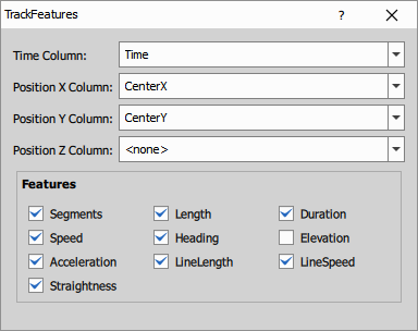
Track feature calculation
Track Features computes track-level summary statistics:
Per-track features:
- Segments: Number of frames in the track
- Length: Total path length traveled
- Duration: Time span of the track
- Speed: Mean, min, max speed
- Heading: Overall direction consistency
- Acceleration: Mean acceleration magnitude
- LineLength: Straight-line distance from start to end
- LineSpeed: Displacement divided by duration
- Straightness: LineLength / Length (1 = perfectly straight, 0 = highly curved)
These aggregate features characterize the overall behavior of each particle.
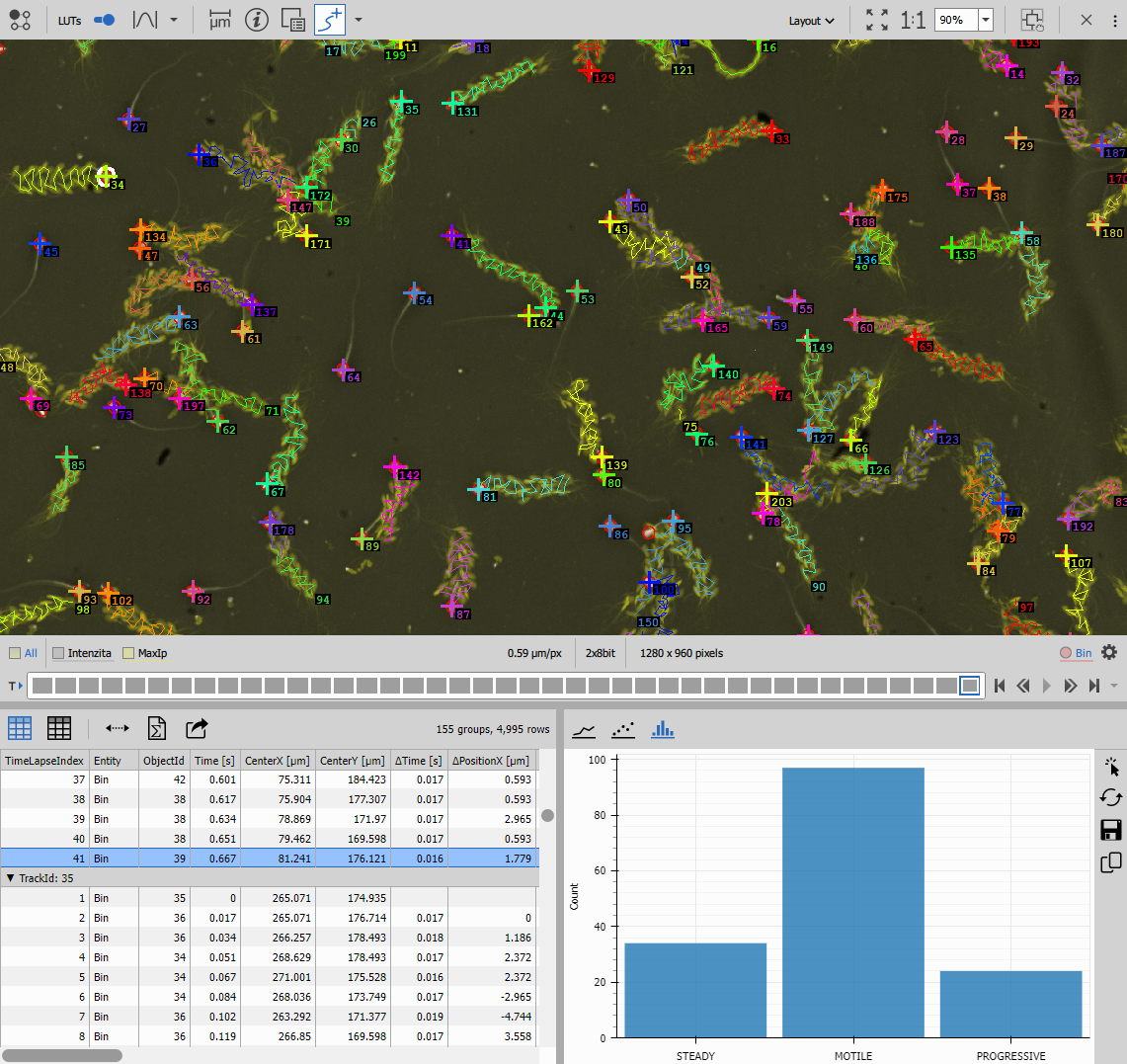
Motility classification
Create Column creates a calculated column classifying tracks by motility:
Classification logic:
Speed < 30 ? "STEADY" : (Straightness < 0.4 ? "MOTILE" : "PROGRESSIVE");This produces three categories:
- STEADY: Low speed, minimal movement (confined or stationary)
- MOTILE: Higher speed but non-directional (random/diffusive motion)
- PROGRESSIVE: High speed and directional (directed migration)
The thresholds are adjusted based on the biological system.
Group by motility
Group Records aggregates tracks by their motility classification, producing summary statistics for each category (count, mean speed, mean straightness, etc.).
Visualization
Line Chart displays individual particle trajectories color-coded by track.
Scatter Plot 4D shows tracks as points in multidimensional feature space (speed vs. straightness, colored by motility class), revealing population structure.
Histogram shows the distribution of tracks across motility categories (how many steady vs. motile vs. progressive).
Tables display both per-frame motion data and per-track summaries.
Results
This workflow produces:
- Track IDs for all particles
- Instantaneous motion features (speed, direction, acceleration)
- Track summary features (length, duration, straightness)
- Motility classification
- Population statistics by motility class
Use cases: Vesicle transport analysis, cell migration modes, drug effects on motility, distinguishing active vs. passive transport
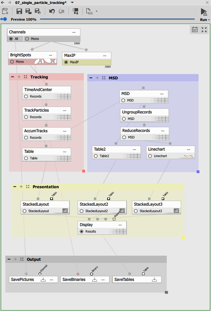
Workflow 3: Single particle tracking with diffusion analysis
This specialized workflow calculates mean squared displacement (MSD) to determine diffusion coefficients, essential for studying Brownian motion and molecular diffusion.
---
config:
  look: handDrawn
  theme: neutral
---
graph TD
  subgraph Tracking
    time[Time and Center]
    track[Track Particles]
    accum[Accumulate Tracks]
    table1[Table - Trajectories]
  end

  subgraph MSD
    msd[MSD]
    ungroup[Ungroup Records]
    reduce[Reduce Records]
    table2[Table - MSD per Δt]
    chart[Line Chart - MSD vs Δt]
  end

  subgraph Presentation
    layout1[Stacked Layout - Left]
    layout2[Stacked Layout - Center]
    layout3[Stacked Layout - Right]
    display[Display]
  end

  subgraph Outputs
    savechn[Save Channels]
    savebin[Save Binaries]
    savetab[Save Tables]
  end

  %% Main workflow
  channels[Channels] -->|Mono| spots[Bright Spots] -->|Mono| time
  channels -->|Mono| maxip[MaxIP]

  time -->|Records - Time, X, Y| track
  track -->|Records - TrackId| accum
  accum --> table1

  %% MSD analysis branch
  accum --> msd
  msd -->|Records| ungroup
  ungroup -->|Records| reduce
  reduce --> table2
  reduce --> chart

  %% Presentation
  table1 --> layout1
  table2 --> layout2
  chart --> layout3

  layout1 --> display
  layout2 --> display
  layout3 --> display

  %% Outputs
  channels -->|All| savechn
  spots -->|Mono| savebin
  display -->|Results| savetab
High-contrast spot detection
Bright Spots detects single fluorescent molecules or particles with stringent settings:
- Diameter: 0.69 microns
- Contrast: 500 (high threshold for bright, well-isolated spots)
- Intensity filters: Remove outliers
These strict criteria ensure only well-localized particles are tracked, critical for accurate diffusion analysis.
Single particle tracking requirements:
- High signal-to-noise ratio
- Isolated particles (no overlap)
- Fast acquisition (short time intervals)
- Stable focus throughout acquisition
Poor localization accuracy will produce incorrect diffusion coefficients.
Tracking for diffusion analysis
Track Particles uses settings optimized for diffusive motion:
Parameters:
- maxSpeed: 4 µm/frame (tight constraint for slowly diffusing particles)
- maxGap: 2 frames
- motionModel: 0 (Brownian motion) - assumes random walk
- stdevFactor: 2.5 - statistical tolerance for position prediction
The Brownian motion model is essential for diffusion studies as it doesn’t assume directional bias.
Long track accumulation
Accumulate Tracks requires:
- MinSegmentCount: 20 frames minimum
Long tracks are necessary for reliable MSD curve fitting. Shorter tracks don’t provide enough data points for accurate diffusion coefficient calculation.
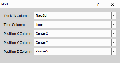
Mean squared displacement calculation
MSD computes the mean squared displacement for each track:
MSD formula:
MSD(Δt) = <[r(t + Δt) - r(t)]²>Where:
- Δt: Time interval (lag time)
- r(t): Position at time t
- < >: Average over all time points and all tracks
The MSD is calculated for increasing time intervals:
- Δt = 1 frame: MSD between consecutive positions
- Δt = 2 frames: MSD between positions 2 frames apart
- Δt = 3 frames: MSD between positions 3 frames apart
- And so on…
Output table structure:
- Δt: Time interval
- MSD: Mean squared displacement at this interval
- StDev: Standard deviation of MSD
- Count: Number of measurements contributing to this point
MSD data processing
Ungroup Records separates the grouped MSD data structure for further analysis.
Reduce Records aggregates MSD values across all tracks, computing:
- Mean MSD: Average MSD at each time lag (the ensemble MSD)
- Count of tracks: Number of tracks contributing
This produces the final MSD curve for the entire population.
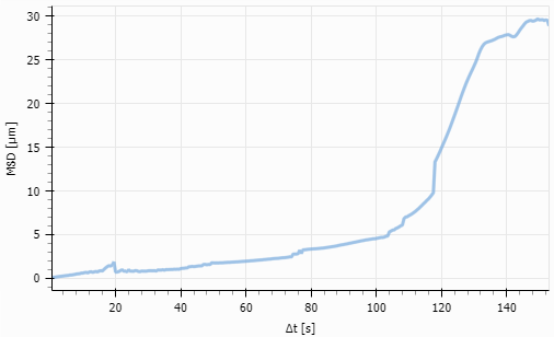
MSD curve visualization
Line Chart plots MSD vs. Δt, displaying:
- The characteristic MSD curve shape
- Error bars showing variability
- Linear or non-linear regime
Curve interpretation:
- Linear MSD(Δt) ∝ Δt: Normal diffusion (Brownian motion)
- MSD(Δt) ∝ Δt^α, α < 1: Subdiffusion (confined or hindered)
- MSD(Δt) ∝ Δt^α, α > 1: Superdiffusion (active or directed)
Diffusion coefficient calculation
For normal diffusion, the relationship is:
MSD(Δt) = 4D·Δt (2D motion)
Where D is the diffusion coefficient.
The slope of MSD vs. Δt gives: Slope = 4D
Therefore: D = Slope / 4
The diffusion coefficient units are typically µm²/s.
Fitting procedure:
- Fit a linear regression to the initial linear region of the MSD curve (typically first 25% of time lags)
- Extract the slope
- Calculate D = Slope / 4
Why only fit the initial region? At long time lags:
- Fewer data points (reduced statistics)
- Boundary effects from finite imaging area
- Photobleaching effects
- Track-to-track variations become dominant
The initial linear region provides the most reliable diffusion coefficient.
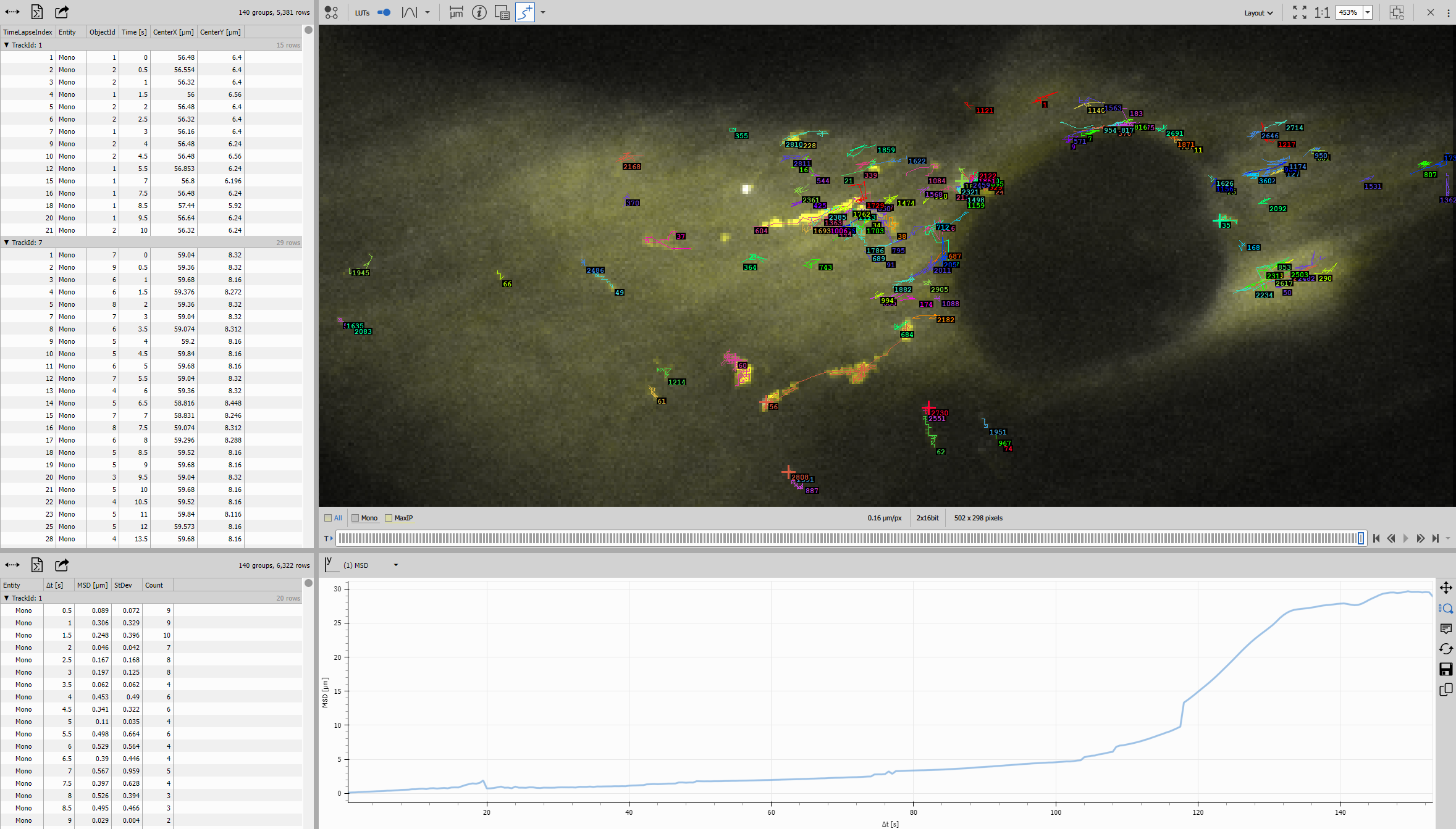
Results interpretation
Tables display:
- Per-track MSD curves
- Ensemble-averaged MSD
- Track counts at each time lag
Diffusion analysis outputs:
- Diffusion coefficient (D)
- Diffusion mode (normal, sub-, or super-diffusion)
- Track statistics (number of tracks, track lengths)
Use cases:
- Molecular diffusion in membranes
- Protein mobility in cells
- Nanoparticle diffusion
- Drug molecule tracking
- Lipid raft dynamics
- Receptor diffusion studies
Comparing the three approaches
When to use each workflow
| Workflow | Best for | Key output | Typical application |
|---|---|---|---|
| Track moving objects | Cells, large objects | Track ID + morphology | Cell migration, growth, division tracking |
| Particle tracking + motion | Vesicles, organelles | Motion features + classification | Transport analysis, motility screening |
| Single particle + MSD | Molecules, nanoparticles | Diffusion coefficient | Membrane dynamics, molecular mobility |
Parameter comparison
| Parameter | Moving Objects | Particle Motion | Single Particle MSD |
|---|---|---|---|
| Segmentation | Cellpose (AI) | Bright Spots | Bright Spots (strict) |
| Tracking method | Track Objects | Track Particles | Track Particles |
| Motion model | Shape-based | Directed (1) | Brownian (0) |
| Min track length | 3 frames | 4 frames | 20 frames |
| Key analysis | Morphology | Motion features | MSD curve |
Workflow complexity
Simplest: Track moving objects - straightforward tracking + measurements
Moderate: Particle motion - adds motion feature calculations and classification
Advanced: Single particle MSD - requires careful acquisition and specialized analysis
Common tracking challenges
Track fragmentation
Problem: Tracks break into multiple segments instead of continuous trajectories.
Causes:
- Objects disappearing temporarily (out of focus, low signal)
- Detection failures in some frames
- maxGap too small
Solutions:
- Increase maxGap parameter (allow longer disappearance)
- Improve segmentation quality
- Optimize acquisition (better focus, higher frame rate)
Incorrect track assignment
Problem: Tracks switch between objects (ID swapping).
Causes:
- Objects too close together
- maxSpeed too large (allows impossible jumps)
- Similar object appearance
Solutions:
- Reduce object density (lower seeding)
- Decrease maxSpeed for more conservative linking
- Use object shape information (Track Objects instead of Track Particles)
Too many short tracks
Problem: Most tracks only last a few frames.
Causes:
- High object turnover (appearing/disappearing)
- Poor segmentation consistency
- Photobleaching
Solutions:
- Increase MinSegmentCount to filter short tracks
- Improve segmentation robustness
- Reduce imaging intensity to minimize photobleaching
- For MSD: reduce required MinSegmentCount if necessary, but interpret results cautiously
Missing tracks at image boundaries
Problem: Tracks end when objects reach image edges.
Causes:
- Objects leaving field of view
- Border effects in tracking
Solutions:
- Use Remove Touching Frame to exclude border objects
- Acquire larger field of view
- Track only central region if migration is non-directional
Best practices
Experimental design
Imaging parameters:
- Frame rate: Fast enough to capture motion (maxSpeed/2 is a guideline)
- Total duration: Long enough for meaningful statistics (10-20x typical track length)
- Field of view: Large enough to capture full trajectories
- Z-position: Maintain focus (use autofocus for long acquisitions)
Sample preparation:
- Density: Moderate density (avoid overcrowding)
- Labeling: Bright, stable fluorophores
- Media: Minimize drift and evaporation
Tracking parameter optimization
Iterative approach:
- Start with default parameters
- Visualize tracks overlaid on images
- Identify problems (fragmentation, swapping, missing tracks)
- Adjust parameters accordingly
- Re-run and verify improvement
Key parameters to tune:
- maxSpeed: Set to 1.5-2× maximum expected speed
- maxGap: Start with 2, increase if detection is inconsistent
- MinSegmentCount: Balance between statistics and data retention
Quality control
Verify tracking quality:
- Visual inspection of trajectories on images
- Check track length distribution (should have a clear peak)
- Monitor track start/end events (should not all be at boundaries)
- Compare forward and backward tracking (should give similar results)
For MSD analysis:
- Examine individual track MSDs before averaging
- Verify linearity in the initial region
- Check that enough tracks contribute to each time lag
- Compare D values across replicates for consistency
Advanced topics
3D tracking
All tracking methods extend to 3D with appropriate inputs:
- Use 3D segmentation (Bright Spots 3D, Threshold 3D)
- Track Particles works with X, Y, Z coordinates
- MSD formula becomes: MSD(Δt) = 6D·Δt (3D motion)
Multi-color tracking
Track particles in multiple channels simultaneously:
- Segment each channel separately
- Track each population independently
- Analyze interactions between populations
Tracking with division
For cells that divide:
- Use specialized cell tracking nodes
- Track lineage relationships (mother-daughter)
- Analyze division timing and frequency
Confined diffusion analysis
For MSD curves showing plateaus:
- Fit confined diffusion models
- Extract confinement radius
- Determine confinement strength
Exporting and further analysis
Results can be exported for external analysis:
Track data:
- Full trajectory tables (X, Y, time, track ID)
- Track summary statistics
- Motion feature tables
For publications:
- High-resolution trajectory images
- MSD curves with error bars
- Statistical comparisons between conditions
Troubleshooting summary
| Issue | Likely cause | Solution |
|---|---|---|
| Tracks too short | Segmentation inconsistent | Improve segmentation, increase maxGap |
| Track swapping | Objects too close | Reduce density, decrease maxSpeed |
| Missing tracks | Detection failures | Optimize segmentation threshold |
| Non-linear MSD | Not normal diffusion | Use appropriate diffusion model |
| Noisy motion features | Low temporal resolution | Use rolling average smoothing |
| Few tracks survive filtering | MinSegmentCount too high | Reduce minimum track length |
Related workflows
- Object counting - Basic object detection
- Time measurement - Temporal measurements without tracking
- Cell measurement - Cell morphology analysis
- 3D counting and tracking - Extension into 3D