Object counting

Object counting is the most fundamental measurement workflow in GA3. At its core, it requires only two steps: segmentation to detect objects and object count measurement to quantify them.

However, this workflow demonstrates a complete analysis pipeline that produces comprehensive results including temporal trends, per-object features, and synchronized visualizations.

What this workflow produces

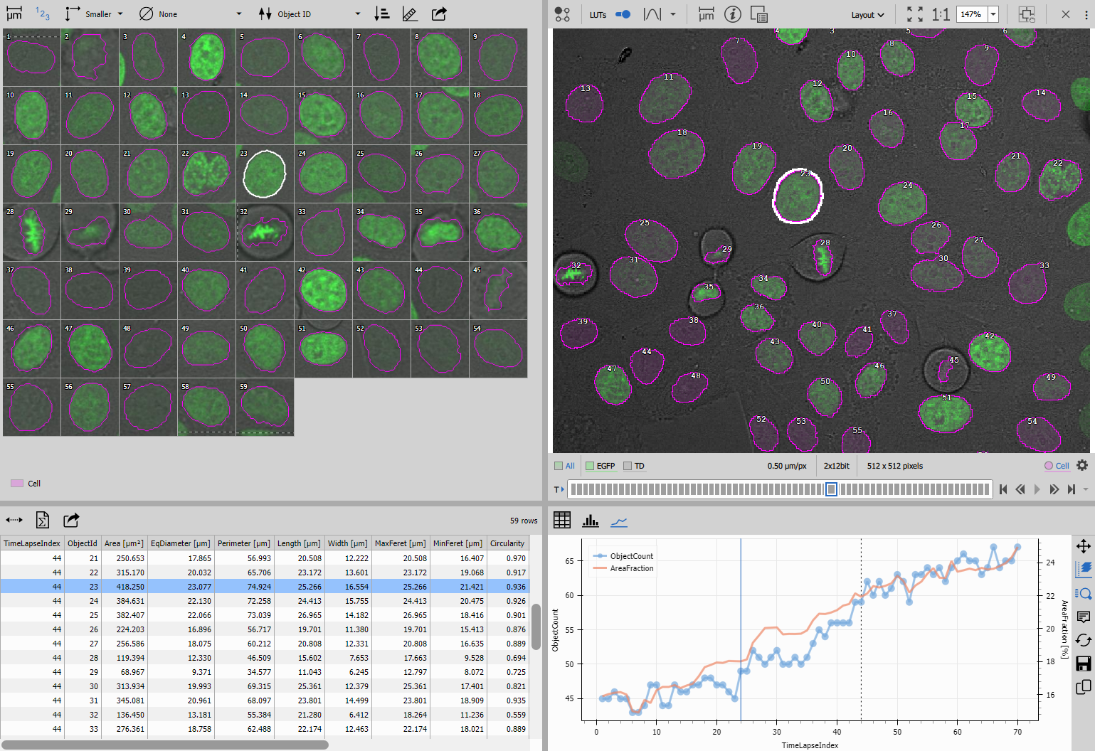
This workflow creates a complete analysis package:

• Per-field statistics table: Object count, total area, and area fraction for each frame in the time-lapse
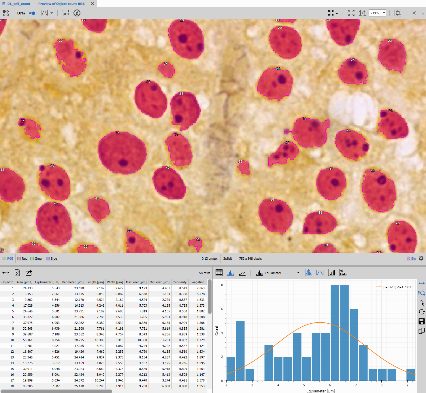
• Per-object features table: Morphological measurements for every detected object in the current frame
• Temporal trend graph: Line chart showing how object count and area fraction evolve over time
• Feature distribution histogram: Shows the distribution of any selected object feature
• Synchronized interface: Links all visualizations to the image, enabling interactive exploration

The result provides both population-level statistics (field counts over time) and individual-level data (per-object measurements).

Workflow overview

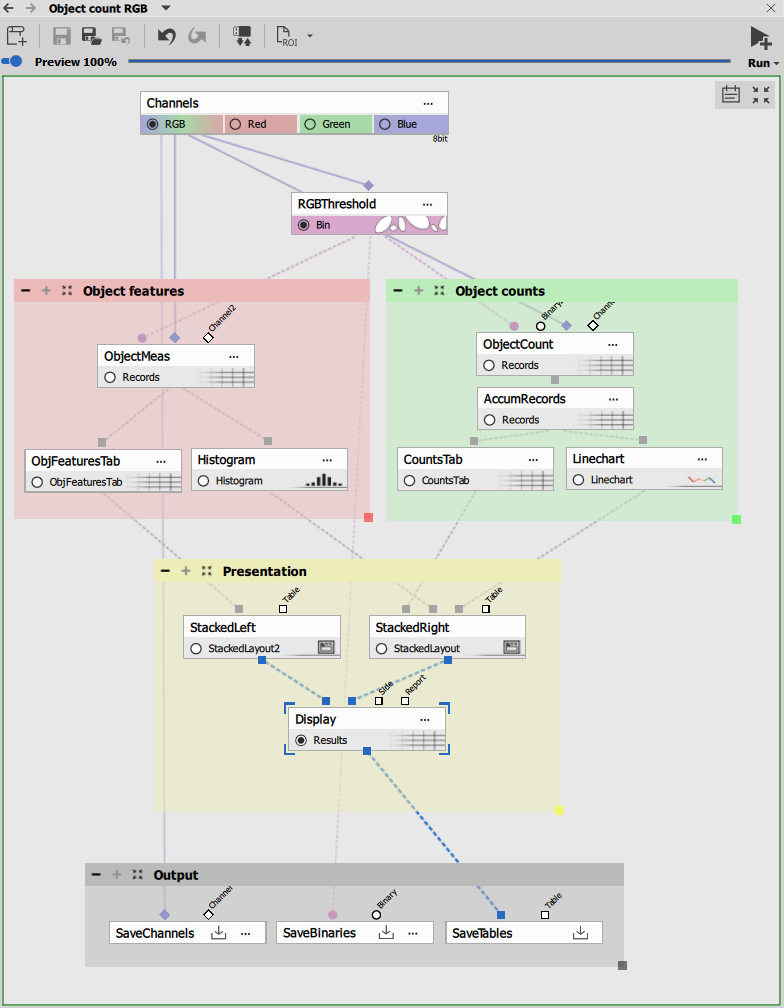
The recipe consists of four functional blocks:

Recipe variations

This workflow comes in three variations that share the same core structure:

RGB version (single frame):

• Uses RGB Threshold for color images
• Processes a single RGB image
• Demonstrates the basic workflow structure

Fluorescence version (time-lapse):

• Uses Threshold for fluorescence channels
• Processes multi-frame time-lapse data
• Shows temporal evolution of object counts

Catalog version (with gallery):

• Adds Object Catalog node
• Displays a grid gallery of detected objects
• Includes border object removal for cleaner results

  
---
config:
  look: handDrawn
  theme: neutral
---
graph TD
  subgraph "Object counting"
    objcount[Object Count]
    accum[Accumulate Records]
    countstab[Table - All Frames]
    linechart[Line Chart]
  end

  subgraph "Object measurement"
    objmeas[Object Features]
    objtab[Table - Current Frame]
    histo[Histogram]
  end

  subgraph "Presentation"
    left[Stacked Layout - Left]
    right[Stacked Layout - Right]
    display[Display]
  end

  subgraph Outputs
    savechn[Save Channels]
    savebin[Save Binaries]
    savetab[Save Tables]
  end

  %% Main workflow
  channels[Channels] -->|RGB or Fluo| threshold[Threshold] -->|Bin| objcount
  channels -.->|All| objcount
  threshold -->|Bin| objmeas
  channels -.->|All| objmeas

  %% Object counting flow
  objcount -->|Records| accum
  accum -->|Records| countstab
  accum -->|Records| linechart

  %% Object measurement flow
  objmeas -->|Records| objtab
  objmeas -->|Records| histo

  %% Presentation
  objtab --> left
  countstab --> right
  histo --> right
  linechart --> right

  left --> display
  right --> display

  %% Outputs
  channels -->|All| savechn
  threshold -->|Bin| savebin
  display -->|Results| savetab

Segmentation

Segmentation is the critical first step that determines which pixels belong to objects of interest. GA3 provides multiple segmentation methods, with thresholding being the most straightforward.

Threshold methods

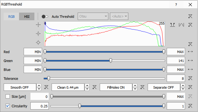
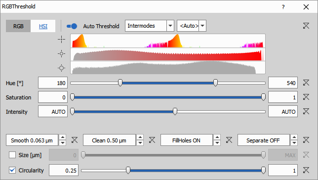
For RGB images - RGB Threshold:

• Works directly on RGB color images
• Separates objects based on color (hue, saturation, intensity)
• Settings used:
  • Auto Threshold Method: Intermodes algorithm
  • IsHSI: 1 (uses HSI color space instead of RGB)
  • GreenHigh: 142 (upper limit on green channel in HSI)
  • Clean: 0.504 µm to remove small debris
  • Smooth: 0.063 µm to regularize boundaries
  • Fill: Enabled to fill holes inside objects
  • FilterByCircularity: Enabled with CircularityLow: 0.25 to remove elongated artifacts

For fluorescence images - Threshold:

• Works on grayscale fluorescence channels
• Separates bright objects from dark background
• Settings used:
  • Auto Threshold Method: Triangle algorithm
  • AutoThresholdOn: Enabled for automatic threshold determination
  • Clean: 0.498 µm to remove noise
  • Separate: 0.498 µm to split touching objects
  • Smooth: 0.498 µm to smooth boundaries
  • Fill: Enabled to fill holes
  • IntensityLow: 114 (manual override if needed)

Alternative segmentation methods

While thresholding works for many samples, GA3 offers more sophisticated segmentation for challenging cases:

Spot Detection:

• For small, bright, round objects (cells, particles, nuclei)
• Uses contrast and expected diameter
• More robust to background variations

Segment.ai:

• AI-powered segmentation for complex structures
• Learns from training data
• Handles variable morphology

Segment Object.ai:

• AI segmentation for specific object types
• Pre-trained models available
• Best for cells, nuclei, organoids

Cellpose:

• State-of-the-art cell segmentation
• Works without training data
• Excellent for cells and nuclei

Choose the segmentation method that best matches your sample characteristics.

Object counting block

This block measures field-level (population) statistics and tracks them across time. It produces a table showing how object counts change over the time-lapse sequence.

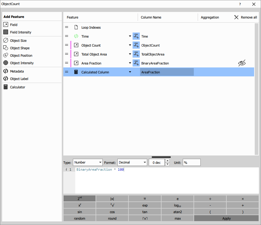
Object Count measurement

Object Count computes aggregate statistics for all objects in each field. Unlike measuring individual objects, this node produces one row per frame containing population-level data.

Measured features:

• Time: Timestamp of the frame (seconds or frame number)
• Object Count: Total number of detected objects in the field
• Total Object Area: Sum of all object areas (µm²)
• Area Fraction: Proportion of the field covered by objects (0-1)

Calculated feature:

• Area Fraction %: Calculated column = AreaFraction × 100 for easier interpretation as percentage

The node has two inputs:

• Binary layer: The segmentation result defining objects
• Channel: For intensity measurements in the objects

This measurement runs frame-by-frame through the time-lapse, producing one row per frame.

Accumulate Records

Accumulate Records collects measurements from all frames into a single table. Without accumulation, only the current frame’s data would be available.

Key settings:

• LoopName: “All loops” (accumulate over all loops - time-lapse, z-stack, multi-point)
• PreviewMode: OFF (accumulate all data in preview)

The accumulated table contains one row per frame, allowing temporal analysis of the entire sequence.

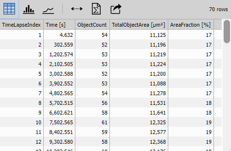
Counts Table

Table displays the accumulated object counts with interactive functionality.

Configuration:

• Data/Display: “All data” to show all frames
• Interaction/Row selection: Enabled to link table rows to image frames
• Statistics: Shows min, max, mean of all columns

Interactive behavior:

• Clicking a row in the table jumps to that frame in the image
• The current frame is highlighted in the table
• Enables quick navigation through the time-lapse

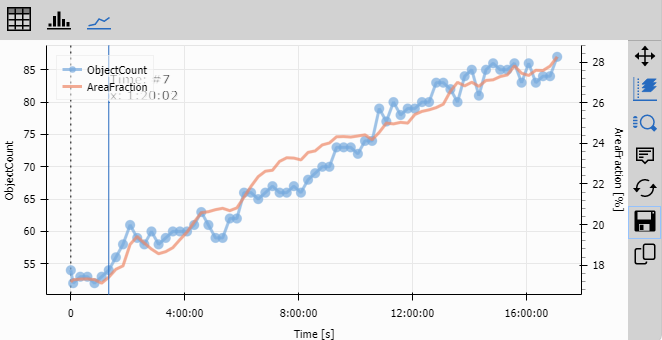
Line Chart

Line Chart visualizes the temporal evolution of object populations.

Configuration:

• Data/Display: “All data” to plot all frames
• X-axis: Time (with format set to display as time)
• Left Y-axis: Object Count
• Right Y-axis: Area Fraction % (secondary axis for different scale)

Display features:

• Dual Y-axes allow plotting variables with different scales
• Time formatting displays timestamps properly
• Interactive tools: pan, zoom, frame selection

This chart immediately reveals trends like:

• Increasing object counts (proliferation, accumulation)
• Decreasing counts (cell death, removal)
• Periodic patterns (division cycles)
• Sudden changes (experimental interventions)

Object measurement block

While the counting block provides population statistics, this block measures detailed features for every individual object. It produces rich morphological and intensity data for single-object analysis.

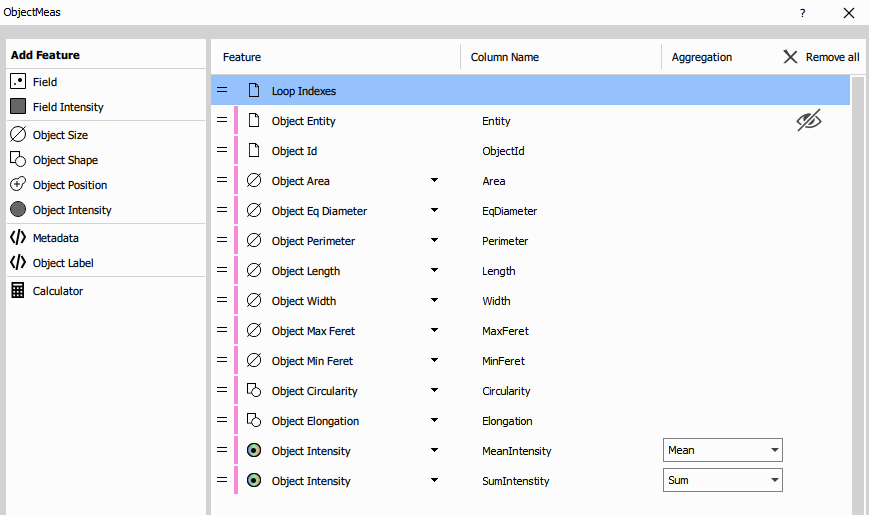
Object Features measurement

Object Features measures comprehensive features for each detected object. This node produces one row per object, with many measured columns.

Inputs:

• Binary layer: Defines object boundaries
• Channel(s): For intensity measurements

Measured feature categories:

Morphological features:

• Size: Area, Equivalent Diameter, Perimeter
• Shape: Length, Width, MaxFeret, MinFeret
• Form factors: Circularity, Elongation
• Position: CenterX, CenterY (object centroids)

Intensity features (per channel):

• MeanIntensity: Average pixel intensity in the object
• SumIntensity: Total intensity (integrated)
• MinIntensity, MaxIntensity: Intensity range
• StdDevIntensity: Intensity variation

This measurement runs per frame, producing a table of objects for the currently displayed frame.

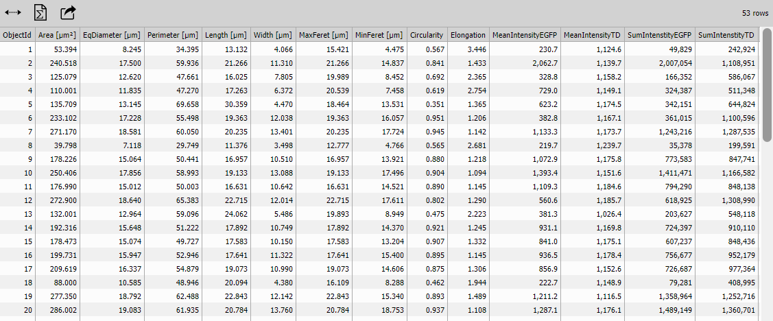
Object Features Table

Table displays individual object measurements.

Configuration:

• Data/Display: “Current frame” to show only objects in the displayed frame
• Interaction/Row selection: Enabled to highlight objects
• Column Sorting: Enabled for sorting by any feature

Interactive behavior:

• Selecting a row highlights the corresponding object in the image
• Selecting an object in the image highlights its row in the table
• Sort by any column to find largest/smallest/brightest objects
• Multiple row selection highlights multiple objects

This enables detailed inspection: “Which object has the largest area?” “What are the intensities of the brightest objects?”

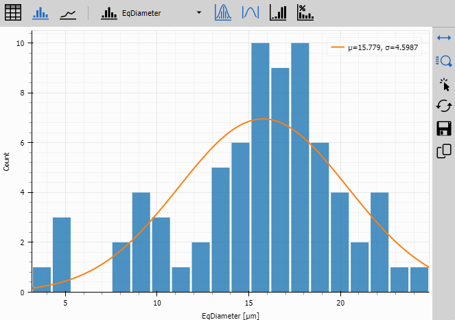
Histogram

Histogram shows the frequency distribution of any selected object feature.

Configuration:

• Data/Display: “Current frame” to show distribution for current frame objects
• Data/Displayed columns: Configurable feature selection (dropdown)
• Bin count: Number of histogram bins
• Fit normal: Optional Gaussian fit overlay

Visualization options:

• Select which feature to plot (Area, Circularity, Intensity, etc.)
• View distribution shape (normal, bimodal, skewed)
• Identify outliers or subpopulations
• Statistical fit shows mean and standard deviation

The histogram reveals patterns like:

• Uniform population (narrow distribution)
• Size heterogeneity (broad distribution)
• Two populations (bimodal distribution)
• Outliers (isolated bars far from the main peak)

Presentation block

The presentation block organizes all tables and graphs into a synchronized, interactive display. This creates a cohesive analysis interface where all views are linked together.

Layout structure

The presentation uses two Stacked Layout nodes to organize visualizations:

Left pane:

• Object Features Table (current frame individual objects)

Right pane (stacked vertically):

• Counts Table (all frames population statistics)
• Histogram (feature distribution)
• Line Chart (temporal trends)

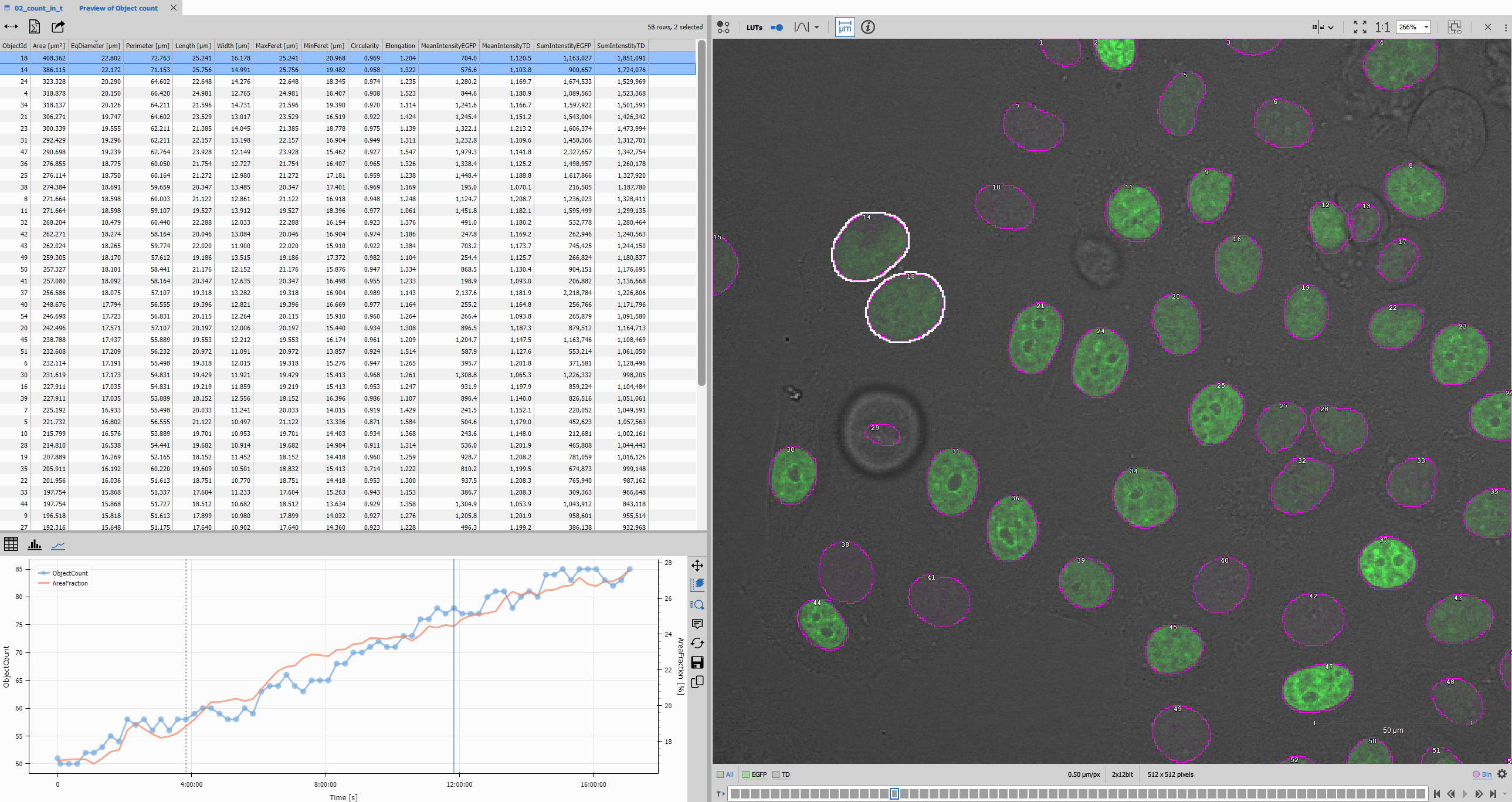
Display node

Display combines the two layout panes with the image viewer.

Settings:

• showNotes: 0 (hides the notes panel)

Synchronized interactions:

• Selecting an object in the image → highlights its row in Object Features Table
• Selecting a row in Object Features Table → highlights the object in the image
• Selecting a row in Counts Table → navigates to that frame
• All views update together when changing frames

The Display node creates a complete analysis environment where image data and measurements are tightly integrated.

Layout customization

The layout button in the interface allows reorganizing views:

• Horizontal or vertical splits
• Resize panes by dragging dividers
• Show/hide individual views
• Maximize specific views

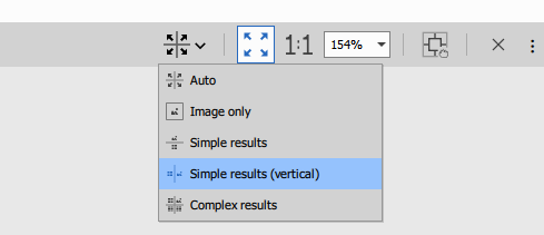
Experiment with layouts to find the arrangement that best suits your analysis workflow.

Output files

The recipe saves three types of output for further analysis or documentation:

Save Channels

Save Channels doesn’t modify channel data as it “stores” the source (Original):

• All input channels (RGB or fluorescence)
• Original intensity values preserved

Save Binaries

Save Binaries saves the segmentation results:

• Binary layers are saved into H5 file by default
• Useful for verifying segmentation quality

Save Tables

Save Tables saves all measurement results:

• Data is saved into H5 file
• Object count table (population statistics)
• Object features table (individual measurements)
• Can be exported to Excel, CSV for external analysis
• Results section includes all graphs and visualizations

Adding the Object Catalog (optional)

The catalog variation adds a visual gallery of all detected objects, which is especially useful for quality control and classification.

Additional nodes for catalog version

Remove Border Objects:

• Removes objects touching the image frame
• Prevents incomplete objects from appearing in the catalog
• Placed immediately after Threshold

Object Catalog:

• Creates a grid gallery of object thumbnails
• Input: Connected to the object features table
• Settings:
  • tableRowVisibility: “all” to show all objects
  • colorChannelSelection: Enabled for channel selection
  • binaryLayerSelection: Enabled to show segmentation overlay

Modified layout:

• Object Catalog gets its own stacked layout pane
• Typically displayed on the left alongside the object table
• Creates a three-pane layout: Catalog | Table | Counts/Charts

Interactive features:

• Click a thumbnail to select that object in the image
• Thumbnails show the object cropped from the original image
• Can toggle between channels and binary overlay
• Useful for visual inspection of segmentation quality

The catalog is particularly valuable when:

• Verifying segmentation accuracy across many objects
• Identifying misclassified objects
• Finding objects with specific morphologies
• Quality control in automated screening

Extending the workflow

This basic counting workflow can be extended in many ways:

Add classification:

• Use feature thresholds to classify objects (small/large, dim/bright)
• Create calculated columns for classification logic
• Color-code objects by class

Add tracking:

• Connect objects across time using Track Objects
• Measure per-track features instead of per-frame
• See Tracking workflow

Add multi-well analysis:

• Process well-plate data with Wellplate Metadata
• Compare object counts across wells
• See Well-plate assays workflow

Add statistical analysis:

• Calculate p-values between conditions
• Fit curves to temporal data
• Use statistical nodes in Data manipulation category

Add 3D analysis:

• Replace 2D threshold with Threshold 3D
• Use Object 3D Count
• See 3D counting workflow

Related workflows

• Time measurement - Temporal measurements without individual object detection
• Cell measurement - Advanced cell morphology analysis with nucleus and cytoplasm
• Tracking - Connect objects across time
• Well-plate assays - High-throughput screening applications
• 3D counting - Volumetric object counting

Summary

Object counting is the foundational workflow in GA3 that demonstrates the complete analysis pipeline: segmentation → measurement → accumulation → visualization. While simple in concept (just threshold + count), this workflow teaches the essential patterns used in more complex analyses:

• Frame-by-frame vs. accumulated processing
• Current frame vs. all data display modes
• Field-level vs. object-level measurements
• Synchronized multi-view interfaces

Master this workflow and you’ll understand the building blocks for all GA3 analyses.